Introduction
Pixel-based visualizations are a very effective way of displaying large datasets in one view. We use it for displaying traffic information, or more specifically: the speed and flow of vehicles from The Hague to Rotterdam during a period of 9 days. The resulting data visualization shows patterns, trends over time, and anomalies.
This is the third post in a series of three on building a pixel-based visualization of traffic data. Part 1 (Introduction and getting data) can be found here, Part 2 (Positioning Pixels) can be found here. This third post looks at color schemes, explains why rainbow color schemes are in general not suitable for data visualization and why we use it anyway for our pixel plot.
Harmful Rainbows
Rainbows are pretty in the sky but can be misleading when used as a data visualization color scheme. See these publications: How the Rainbow Color Map misleads, The End of the Rainbow?, Rainbow Color Map (Still) Considered Harmful.
This is especially true when visualizing numerical or ordinal data, i.e. data that has an intrinsic order (like temperature or ratings of restaurants). The colors of the rainbow however have no intuitive order: is red – green – blue the correct order, or is it red – blue – green? The image below shows that working with gradients (color scheme 2) is much more intuitive, it is immediately clear that [b] shows the data ‘in order’ and [a] does not. Note that even the order is more clear in color scheme 2, it is still not clear whether [b] depicts the order from high to low, or from low to high (we will come back to that later).
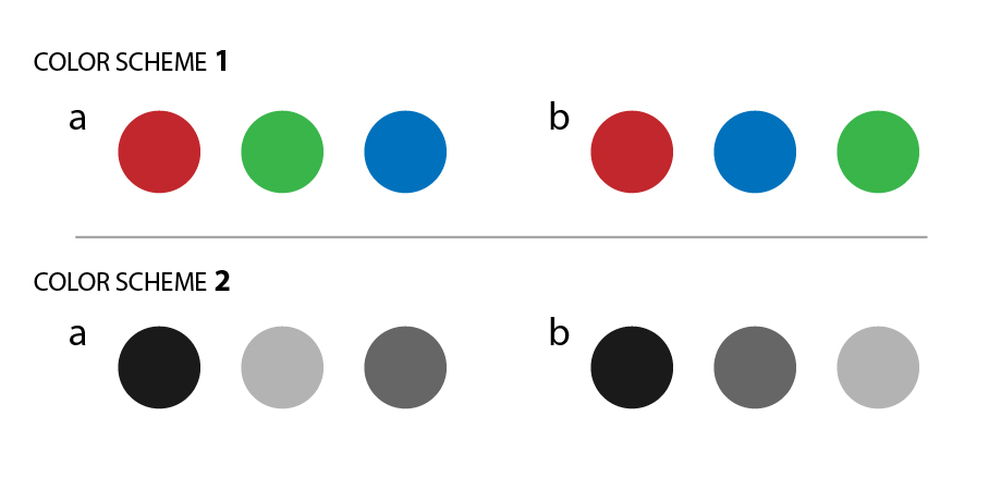
Two color schemes, one based on ‘rainbow colors’, the other using a gradient. Color scheme 1 has no intuitive ordering, in color scheme 2 the order is immediately visible.
When using the rainbow color scheme for continuous numerical data, there is another issue with the rainbow color map. Imagine that the image below is a visualization of some numerical property with its value changing gradually from high (red) to low (purple). While the value changes gradually, the colors do not! There seem to be ‘bands of colors’ with sharp changes in between, which incorrectly suggest sudden changes in values in the underlying data.

Rainbow colors, representing gradually changing values. The color range however, shows sharp changes in color, not present in the underlying data.
In our case however, we did choose to use (part of) the rainbow color scheme because people easily associate green, yellow, and red to traffic speeds. They intuitively map green to ‘fast’, yellow to ‘slower’, and red to ‘very slow, or standing still’ in analogy to traffic lights. Google traffic uses that same color scheme. The downside of this color scheme is that subtle changes in traffic speed are lost because different shades of green and red are relatively hard to distinguish. So in fact we are using it more as a categorical color scheme than a continuous one.
If we would however focus more on the continuous aspect of our data to show the subtle changes in speed, rather than just the categories ‘slow’, ‘slower’, ‘very slow’, we probably would use a color map that gradually changes its hue and brightness at the same time. A good starting point are the color maps shown below, designed by Stéfan van der Walt and Nathaniel Smith for MatplotLib. The code for generating them can be found here.
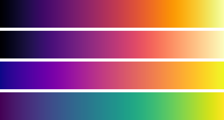
Color maps that gradually change both hue and lightness. From top to bottom: inferno, magma, plasma and viridis. See also https://bids.github.io/colormap/
Let’s compare a few of the mentioned color scheme’s on our traffic data.

Green-yellow-red
This color scheme takes a subset of the rainbow-color scheme, using only the color range green-yellow-red. We choose those colors since they have a semantic connotation with fast, medium and slow traffic. Since the colors we use have a clear meaning in the traffic domain, this scheme does not suffer from non-intuitive order of colors (as described above). However, it still suffers from non-gradually changing colors and brightness. Within the green values hardly any variation is visible, while the change to yellow is sudden and abrupt.

Rainbow
Here we use the full spectrum of colors. Since we use more colors than in the original color scheme (green-yellow-red), values that are close together will still be distinguishable here, where they may not be distinguishable in the original version. So the rainbow color scheme will show more detail, and subtle changes will be better visible here than in the original version. However, the semantic mapping is bad: red still means very slow, but green is medium speed, and purple is fast. In addition, the rainbow scheme has some inherent problems that we pointed out earlier: no intuitive order of color, and sharp changes between colors.

Plasma
This color scheme does not have the problems of the rainbow scheme. It changes gradually in brightness (from purple to yellow), and does not have sudden changes in color: the hue changes very gradually as well. Changes in speed will therefore be reflected better (i.e. more truthfully). Used on traffic data however, this scheme is semantically less intuitive than the green-yellow-red mapping.

Viridis
The Viridis color scheme has the same advantages as the Plasma scheme: gradually changing hue and brightness, resulting in accurate representation of changes in data. It only ‘travels’ a different route through the color cube, resulting in yellow-green-blue instead of yellow-orange-purple. So whether to choose Plasma or Viridis is mainly a matter of taste, unless one of the color schemes better matches the association between color and data that users may have.
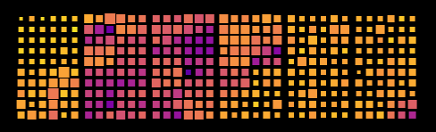
The color schemes that seems to be most suitable for our traffic data are the green-yellow-red scheme (because of its clear connotation with fast, medium, and slow) and the plasma/viridis color schemes (because they show subtle changes better than the rainbow-color-based scheme’s, and are therefore a more accurate representation of the underlying data). The image below shows the Plasma color scheme (top) and the rainbow-based green-yellow-red (bottom). Some changes in speed are better visible in the Plasma scheme, for instance in the 12:00 block at the far left. As you may have guessed from the first blog-post in this series, we choose to use the Plasma color scheme, for its more accurate representation of the data.
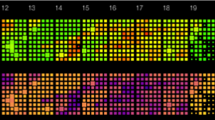
Comparison between rainbow-based color scheme (top) with Plasma color scheme (bottom). Subtle changes in speed are better visible in the latter, while the top scheme has a more intuitive mapping between speed and color (green is fast, red is slow).
Conclusion
This series of posts showed how traffic data can be visualized with pixel-based visualization techniques. We discussed the motive behind this type of visualization and how we retrieved the data (from the NDW, see post 1), It discussed the most optimal way of arranging pixels (a modified Z-order, see post 2) and it showed why we choose the yellow-orange-purple-blue color scheme (this post). Whether this is the best way to visualize remains a topic of further investigation, and requires user tests. These tests will reveal whether users do indeed see interesting patterns and outliers that they would not see with other types of visualization, or that would not be detected with other (e.g. automatic) methods.
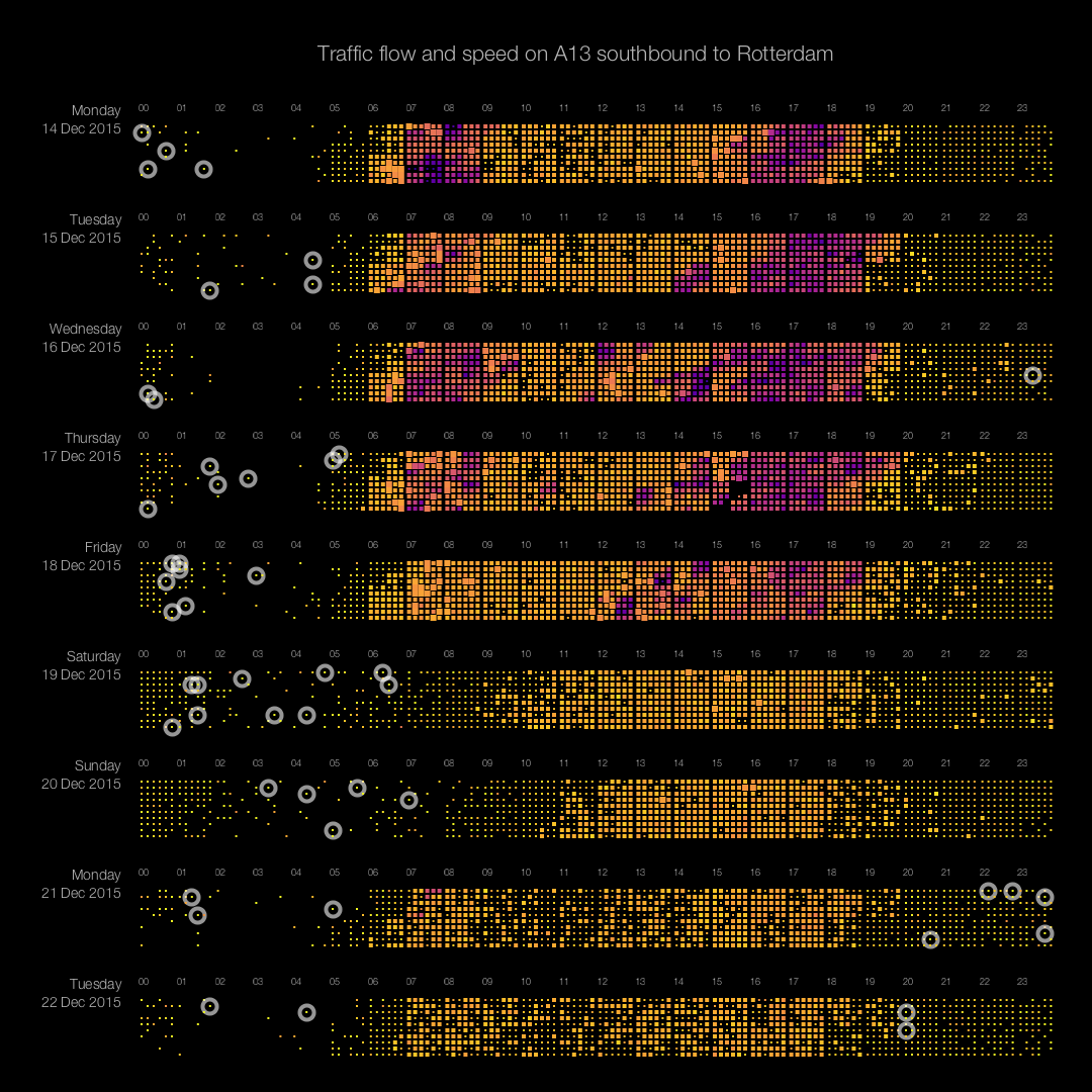
Pixel-plot of traffic data over 9 days on the A13 to Rotterdam. Color indicates speed, rectangle-size indicates flow. Circles highlight speeding cars (driving faster than 150km/h). Click image to open full size version in a new tab.
Recent Comments